Abstract
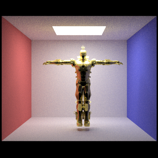
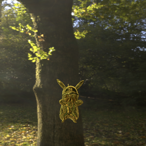
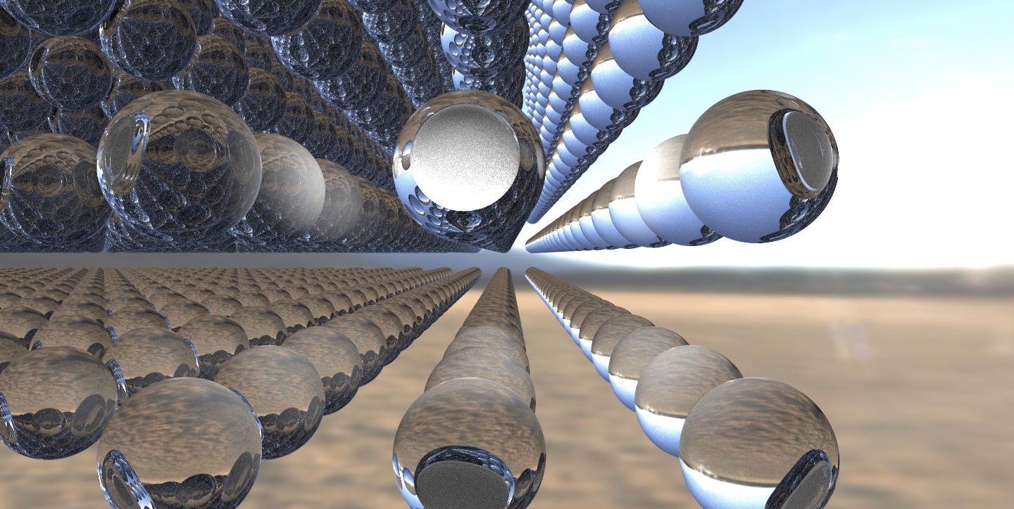
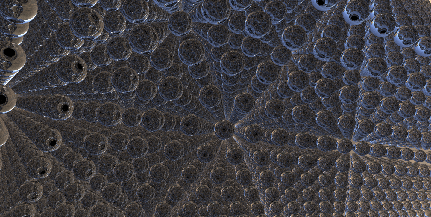
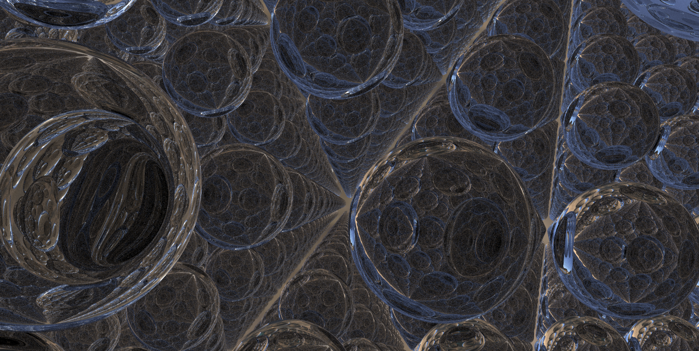
In Project 3-1 and 3-2, we learned the theory and implementation that allowed us to generate some very beautiful, high resolution images through path tracing. However, while the calculations may not be that complicated, the mathematical operations involved along with each rendering’s iterative use of these algorithms are computationally expensive, leading to the slow render times of nearly 30 minutes for a single, relatively more complicated mesh. With modern processors and specialized architecture, specifically the GPU, the tools are available to make path tracing much faster by accelerating the rate at which these calculations are completed. In this context, the Nvidia OptiX Ray Tracing SDK provides a whole host of path tracing functions written in CUDA ready to be run in a GPU context. Our project creates a GPU enabled environment, then refactors and augments Project 3 code to render meshes of much greater difficulty in a much shorter amount of time. Our results reduced render times for Project 3 meshes from several minutes to one or two seconds. Having more powerful computation also allowed us to experiment with more complicated meshes, materials, and environment maps that wouldn’t be accessible in a CPU context. Below, we include rendered object files from both online and self designed, including highly defined characters like Iron Man, Pikachu, and Charmander! We push the upper limits of the GPU capabilities with a render of 15000+ spheres. To our delight, in every instance, the GPU not only completed the mesh in seconds, but also provided real time camera adjustments and afforded us a greater diversity of images we could render. We greatly enjoyed working on this project, and it was such a fulfillment to see formerly intensive images be completed nearly instantaneously. It helped us appreciate the immense role powerful hardware plays in fast and dynamic graphics. Our team highly encourages future 184 students to explore projects in this domain of improving the computational tools for graphics programs and applications.
Final Video
Technical Approach
Part 1: Setting Up GPU Enabled Instance
Amazon Web Services
Create an AWS EC2 instance with an available GPU.
Environment Setup
Install Desktop GUI
Purpose: The Optix code and examples we worked with opens an interactive dialogue containing the image. Setting up a GUI is necessary so that the interactive window opens up and allows us to interact with the rendering.
Ubuntu / Linux Instance
1. SSH into the instance and install the "ubuntu-desktop" and "xrdp" packages. Check that both are installed by running "apt list --installed".2. Edit the Remote Desktop Protocol file at the path "etc/xrdp/xrdp.ini" on the host.
4. Restart RDP with `sudo service xrdp restart`
5. Download Microsoft Remote Desktop from the Mac App Store
6. Add a new desktop. Within the PC Name, enter <Instance's Public IPv4 Address>:3389
Windows Instance
Make sure you have Microsoft Remote Desktop installed. Clicking the "connect" button on the EC2 Instances dashboard will download an RDP file that can be used to connect.
Note: We gave up on AWS because the GPU instance we were using did not have enough RAM for the OptiX SDK.
Google Cloud Platform
Create a Google Cloud instance with an available GPU.Environment Setup
- Request increase GPU instance quota increase from 0 to 1 from Google Cloud. We used an NVIDIA Tesla K80 GPU in the us-west1-b time zone (Oregon area)
- Install associated NVIDIA driver and CUDA with script from Google Cloud documentation
- Install OptiX Toolkit. We used v5.1.0 for Linux as this was the latest version compatible with the K80 GPU
- Install xfce4 Ubuntu display manager (for GUI)
- Install and set up VirtualGL for a headless NVIDIA instance
- Install and set up TurboVNC server
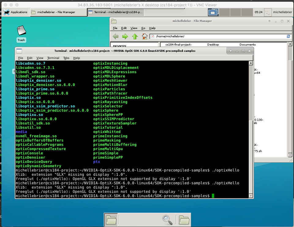
We needed VirtualGL to handle OptiX's OpenGL/GLX dependencies on a headless GPU instance. VirtualGL redirects an application's OpenGL/GLX commands to a separate X server with access to a 3D graphics card, captures the rendered images, and streams them back to the application's X server (explanation taken from the VirtualGL wiki). Initially, we tried not using a GUI at all and just saving the output to a file, but still ran into errors when trying to run the precompiled executables in the SDK as this "save to file" functionality in the SDK samples works by creating an OpenGL context then saving to a file, and we didn't even have a display connected. We then tried using a GUI served by a TightVNC server with the xfce4 display manager, but found that this couldn't handle the GLX commands from the application (see screenshot below).
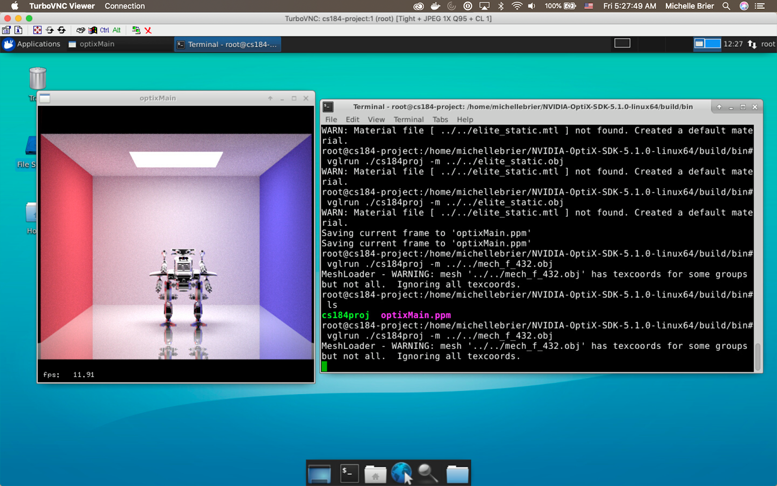
After setting up VirtualGL to run on a headless 3D X server on our GPU instance, we needed a vncserver implentation. Although VirtualGL can provide 3D rendering for any vncserver implentation, including TightVNC, which we initially used to set up the GUI, we switched to TurboVNC as this is specially optimized to have the best performance with VirtualGL. With this, we were able to successfully run interactive 3D renders on our GUI using a Google Cloud GPU (see screenshot below).
Workflow
We ended up only using our Google Cloud instances. After setting everything up, to start up the GUI, we simply had to start the TurboVNC server and connect to the port the display was being served on at the instance's external IP address using a TurboVNC client. To build and make executables, we configured a build folder and ran make. We were
then able to run executables normally on the GUI by prefacing commands with vglrun.
Part 2: Pathtracer Code
To port over the pathtracer functionality from project 3, we added features to a basic pathtracer implementation included in the SDK in
optixPathTracer.cu and optixPathTracer.cpp.
1. Sphere geometry instance
The SDK's pathtracer only included parallelogram geometry instances, with the bounding box and intersections handled in
parallelogram.cu. We needed a sphere geometry instance for the CBspheres rendering from project 3, so we included
a sphere.cu CUDA C file (taken from the SDK) to handle a sphere's bounding box and ray intersections with a sphere. Now, we could create (diffuse surface) sphere geometry instances and place them in our Cornell Box scene in optixPathTracer.cpp, replacing the
old parallelogram instances.
2. Mirror and Glass Closest Hit Handling
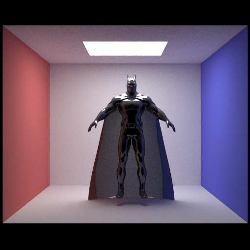
At this point, we could only render diffuse surfaces, so we added closest hit handling for mirror surfaces to the optixPathTracer.cu CUDA C file as well as closest hit handling for glass surfaces. We found NVIDIA's Cg (a high-level
shading language develoepd by NVIDIA) standard library useful here. For the mirror surface closest hit function, we used
the reflect function from the Cg standard library to, given an incidence vector and a normal vector, return
the relection vector. For the glass surface closest hit function, we used Cg's refract
function to, given an incidience vector, a normal vector, and a refraction index, return a refraction vector. For the
rays that weren't refracted (for which refract returned a falsey value), we returned the reflection vector
using reflect.
While implementing this, we looked at the glass implementation in the OptiX advanced samples repo for reference, which didn't use
any Cg functions and rather implemented the mathmatical equations directly, like we did in project 3. However, as the Cg
standard libary seemed to do the same thing, we decided to use these Cg functions in our implementation instead, and found the
result to be satisfactory.
After this, we could create geometry instances with either diffuse, mirror, or glass surfaces, and
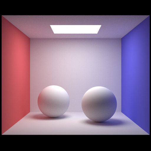
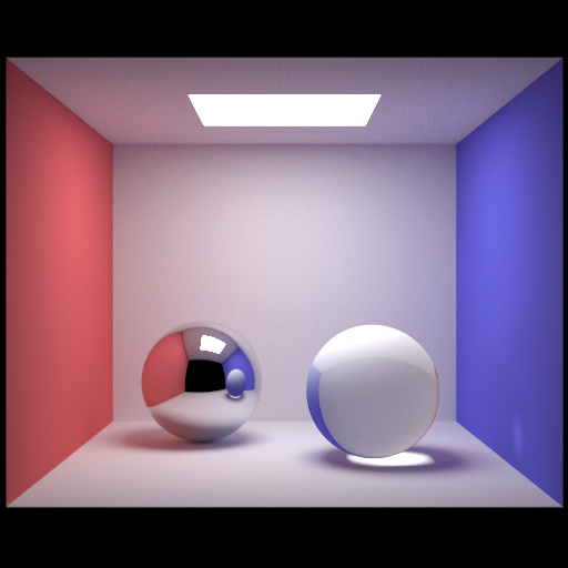
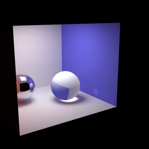
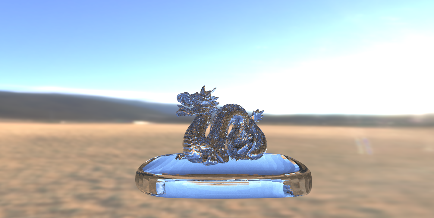
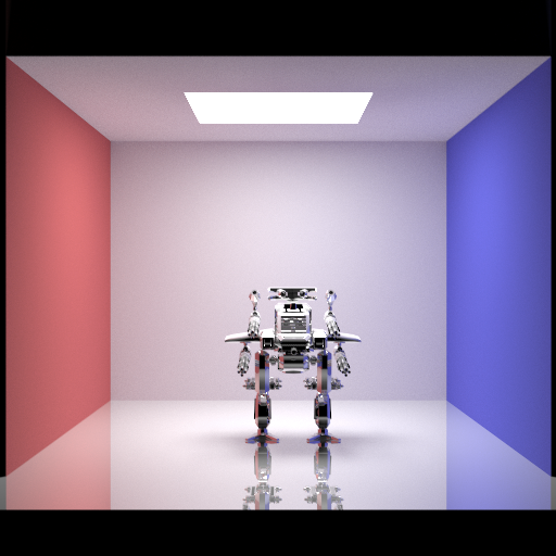
we could render the CBspheres scene from project 3 with a mirror surface ball and a glass ball.
3. Mesh Input Handling
At this point, we could only render a hardcoded Cornell Box scene with geometry instances at hardcorded coordinates, so
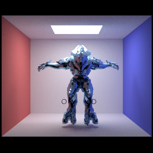
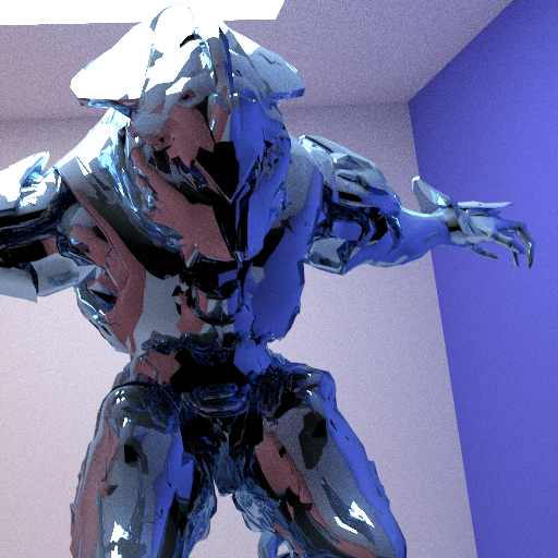
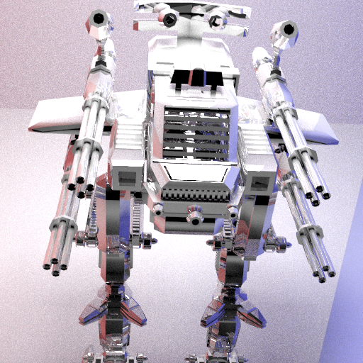
in this step, we added handling for input meshes (in the form of .obj files) passed in with an -m flag. We did this by creating an OptiXMesh instance, applying a material (diffuse, mirror, or glass) to it, and passing it into the OptiX API's loadMesh function along with an affine transformation to correctly adjust the mesh's orientation in the scene (we had a few affine transformations for different renderings, which we simply decided to hardcode, rather passing them in as inputs and handling the input), and along with the file to load from. We then created an axis-aligned bounding box for the mesh (using Aabb.set(mesh.bbox_min, mesh.bbox_max)) and returned a geometry instance created from the OptiXMesh object. We found that in addition to the surface material and color we manually specified in the code for the mesh, if we included a .mtl file in the same directory as the mesh, OptiX automatically mapped the material onto the mesh in the rendering (this was how we got the Halo Elite rendering's surface material, shown in the Results section of this writeup). After completing this, we were able to render custom objects, not just parallelograms and spheres, in the Cornell Box scene. To render more project 3 images, we converted some project 3 .dae files to .obj files to pass in as mesh inputs.
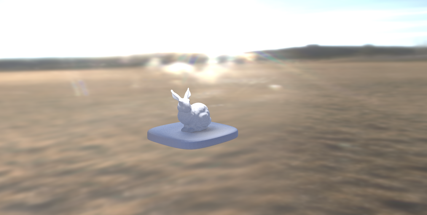
4. Environment Mapping
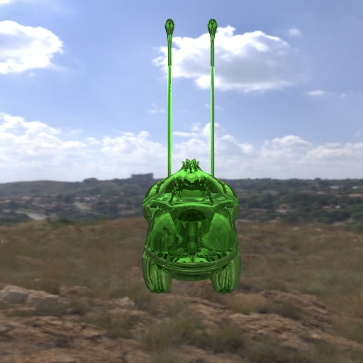
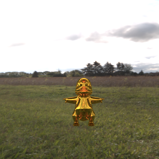
Now, to render scenes other than a Cornell Box, we added environment mapping. We first read in an .hdr file passed in with a -t flag, set the context's envmap variable to a texture sampler created from a texture loaded from the .hdr file passed in (using the OptiX API's loadTexture) function, then changed raytracing misses to sample from the this environment texture map via an envmap_miss function (taken from optixTutorial in the SDK) we added to optixPathTracer.cu. The normal miss function (for non-environment map scenes) was already implemented in optixPathTracer.cu as the miss function. After this, we were able to render any parallelogram, sphere, or mesh geometry instance with an environment map background rather than just a Cornell Box.
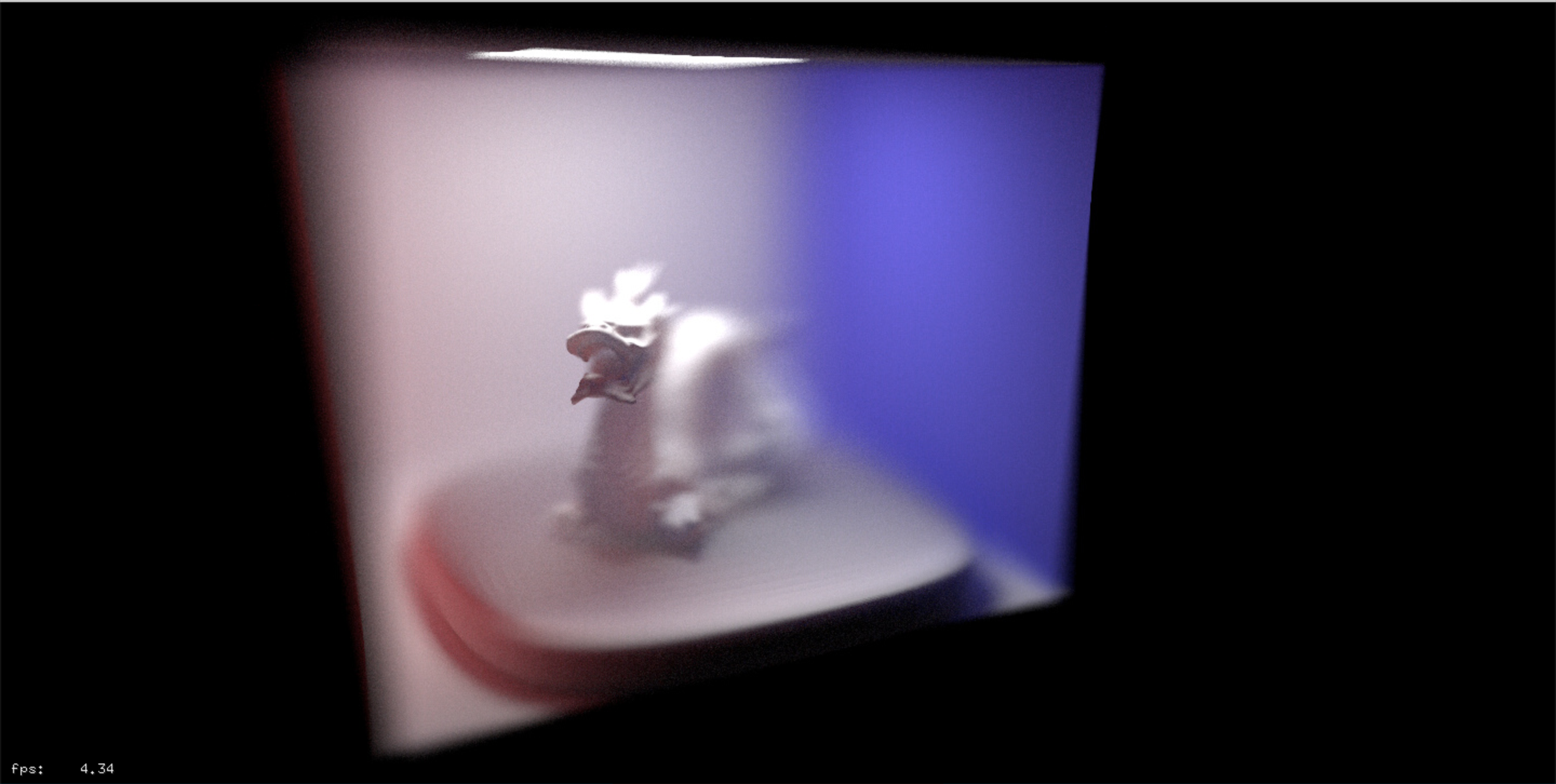
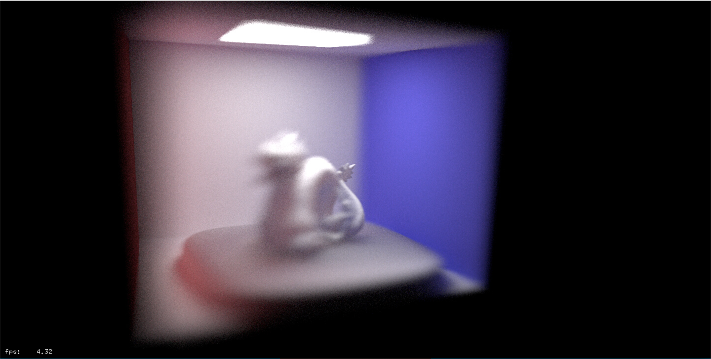
5. Thin Lens Camera
Finally, we implemented a thin lens camera in CUDA C in optixPathTracer.cu to render scenes with depth of field, as the basic pathtracer in the OptiX SDK only used a pinhole camera model. This involved tweaking the existing camera implementation to instead calculate the intersection of the eye ray and the plane of focus (at point pFocus), uniformly sample a point on the disk representing the thin lens (point pLens), then set the ray direction to the normalized direction of the ray from pLens to pFocus, similar to how the last part of project 3-2 was implemented. We also added some additional handling for keyboard presses in optixPathTracer.cpp to toggle increases/decreases in lens radius and focal distance while interacting with the rendering (we've included a video demo of this in the Results section). After this, we were able to render images with depth of field, with the ability to change the aperture size and adjust the focal distance of the camera real-time.
Part 3: Experiment with different BSDFs, materials, meshes, and environment maps
After implementing our desired functionality, we had fun playing around with different material surfaces, surface colors, refraction indexes, meshes, and environment backgrounds to experiment with our new pathtracer, and to generate many of the videos and images we've included in the Results section of this writeup!
Difficulties
We struggled quite a bit in setting up an environment capable of 3D interactive rendering using a GPU instance on a VM. First, we didn't have much experience with Ubuntu, so setting up and configuring the Ubuntu instances with the appropriate drivers and OptiX took some time. Then we had to figure out how to set up a GUI with a display capable of handling OpenGL/GLX commands. Again, due to our relative inexperience with headless instances and Ubuntu, this proved challenging. A few times during this process, we even ran out of memory on our VMs and had to restart from scratch. Overall, it took a frustratingly long time just to get an environment and workflow set up and OptiX compiling. However, after we got past that, it was relatively smooth sailing. The OptiX SDK had plenty of resources, API usage examples, and CUDA files that proved helpful as we were implenting our pathtracer, and the existing scaffolding in optixPathTracer.cpp and optixPathTracer.cu was helpful in improving our understanding of how a basic OptiX pathtracer works and in saving us time having to figure out how to do small, menial things like finding the coordinates to correctly position walls of the Cornell Box together in the scene, as optixPathTracer.cpp already had a hardcorded Cornell Box scene set up. When implementing the thin lens camera, however, it took some time understanding the UVW basis used in OptiX, and we spent a while debugging this.
Lessons Learned
- Configuring a platform is difficult! Setting up the GPU and development environment took way, way more time than we thought.
- For real time camera adjustments, convergence (fuzziness) may take a few seconds, even with a GPU. If we had more time, we would have liked to set up another instance with a more powerful GPU to test the quality and convergence time of renderings, as the Tesla K80 isn't the most powerful NVIDIA OptiX-compatible GPU out there.
- The entirety of our pathtracer with the functionality of the pathtracer we developed in project 3 incorporated/touched files that only made up a small part of the OptiX SDK. If we had more time, exploring the OptiX API could've led to many more rendering possiblities!
Results
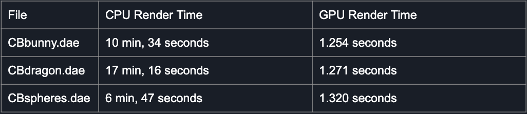
Timing Comparisons
Video Demos
Graphical Results
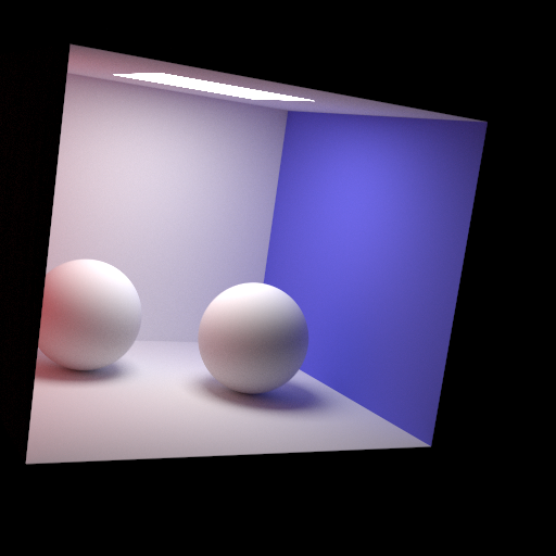
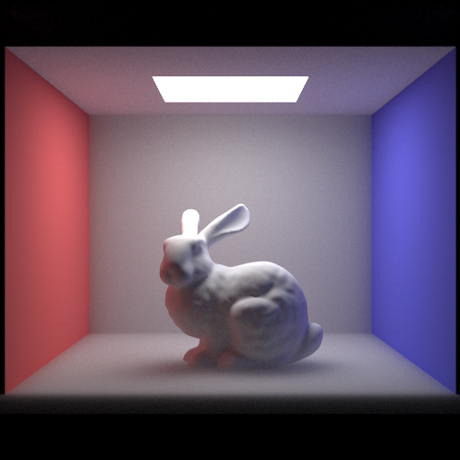
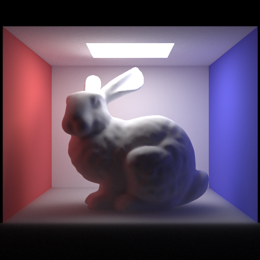
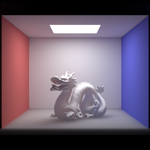
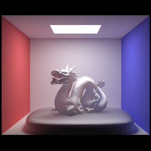
Project 3 Images
|
|
|
|
|
|
|
|
|
|
|
|
Graphical Results
Advanced Images
|
|
|
|
|
|
|
|
|
|
|
|
|
|
Final Presentation Slides
References
Team Member Contributions